Part 2 of a series of 2 posts where I explore how I lost 1000 euros betting on CS:GO with machine learning (ML). This post covers the actual implementation of the solution: CS:GO, feature engineering, modelling, validation, backtesting and lessons learned.
Author
Pedro Tabacof
Published
July 11, 2024
This is a true story of how I lost money using machine learning (ML) to bet on CS:GO. The project was done with a friend, who gave me permission to share this story in public.
Check out the first post of the series, which covers the theory and foundations necessary to understand what’s going on in this second post:
What is your edge?
Financial decision-making with ML
One bet: Expected profits and decision rule
Multiple bets: The Kelly criterion
Probability calibration
Winner’s curse
In this post, I will go over the actual implementation of the solution:
CS:GO basics
Data scraping
Feature engineering
TrueSkill
Inferential vs predictive models
Dataset
Modelling
Evaluation
Backtesting
Why I lost 1000 euros
Solution
Before we get to the actual solution, I need to explain some CS:GO basics:
CS:GO basics
Counter-Strike: Global Offensive (CS:GO) is a first-person shooter (FPS) multiplayer game. It can be played casually or competitively. When played competitively, it’s typically played on the following format:
Two teams of 5 play against each other: Terrorists vs Counter-Terrorists
Best of 3 maps (sometimes best of 1 or 5)
Maps are played up to 30 rounds
Each round can be won be killing the other team or by planting or defusing the bomb
Each player has a number of kills (K), deaths (D), assists (A) and average damage per round (ADR)
If you don’t know much about video-games, don’t worry, you can treat CS:GO as any other competitive team sport: Each match has a winner (in case of best of 1, it could be a tie) and each team and player have stats that correlate with their performance in the match. Teams are composed of players which range in talent, there are star players, dominant teams, and players might change teams over time.
CS:GO score screenshot from https://blog.scope.gg/cs-go-stats-why-is-it-so-important-en/
Web scraping
Data is the new oil.
As I explained in the first post, one of the reasons we chose CS:GO was data availability. Since we might have broken some term and conditions, I won’t name our exact sources, but they were easily found online.
We collected both match data and betting odds. Note that match data is easy to find retroactively, but betting odds need to be collected in real-time, which limited our ability to run backtests (more on this later). Betting odds data is super valuable, and maybe a better way to make money would have been to collect it across different websites and simply sell it1.
We collected 3 years worth of match data over 30k matches. We managed to collect only 3 months of betting odds data, covering 1725 matches, with approximately 30 odds per match. Note that the odds fluctuate between the match announcement and start.
Match data contained information such as the teams playing, team composition, kills and deaths for each player, rounds won, the map to be played, the final score (win-loss-tie), and much more.
To scrape the data that we needed we used Selenium through a headless browser. That was necessary because the website content was dynamically loaded using JavaScript. Then, we parsed the resulting HTML with BeautifulSoup. We would run a batch job every night to get the new match data and old match results. Betting odds, however, were collected more frequently.
Feature engineering
Past behavior is the best predictor of future behavior.
With the match data, we created 100s of features2. Most features were related to past performance, such as the percentage of times team 1 won on the map to be played or against team 2. If the teams faced each other off before, who won back then is an important predictor now. We also used game score features like KD difference and ADR on a team and individual basis.
Note that we couldn’t use the betting odds as features, even though the information there is invaluable3. The reason is simple, as previously explained: we didn’t have a backfill for historical betting odds. We could only use the odds that were available after we started to collect them, which was only (barely) enough for backtesting.
Also, we had a trump card, which ended up generating the most important set of features: TrueSkill.
TrueSkill
TrueSkill is a Bayesian skill rating system developed by Microsoft for multiplayer games, a Bayesian version of the ELO rating. It aims to estimate the “true skill” of each player or team based on their performance history.
TrueSKill uses a Gaussian distribution to represent the skill level of each player, and it updates these skill levels after each match using Bayesian updates4. TrueSkill provides not just the ability but also the uncertainty around each player’s skill, both of which can be used as features in a ML model.
Inferential vs predictive models
There are two cultures in the use of statistical modeling to reach conclusions from data. -Leo Breiman5
If we have TrueSkill, which predicts the win probability between two teams, why do we even need a ML model? TrueSkill is an inferential model, which attempts to explain the world through latent variables. Of course, a perfect model of the world would also make great predictions but, in practice, there is always a trade-off between explainability and predictive power. That is the biggest tension between statistics and ML.
ML models are typically less interpretable black boxes but much more powerful at making predictions. They can incorporate a wide range of features, including but not limited to those provided by TrueSkill, with the sole focus of optimising a loss function, which generally translates into better predictions.
Dataset
Here is the matches dataset with all the features and target together, including the TrueSkill features. I don’t provide the actual feature engineering code for the sake of brevity, as this post is long enough as it is.
The modelling done here is pretty standard tabular ML with a couple of notable exceptions:
We remove ties, which represent roughly 1.5% of the dataset6.
We do data augmentation by swapping team1 and team2 features and adding both rows to the training set
We can do that as there is no “home advantage” in CS:GO like there is in football7
When making predictions, we average the predictions across both scenarios
Out-of-time train-test split
We use out-of-time split instead of the more typical cross-validation. In pretty much any real-life application, a model is trained with past data and then is used to predict future unseen data. Your evaluation should reflect that, as you might be interested to know how your model performance degrades over time (which could be caused, for example, by concept drift). In that sense, almost all ML problems are time series problems and should be evaluated as such8.
dataset['match_date'] = pd.to_datetime(dataset['match_date'])# Create weekly match countsmatch_counts = dataset.groupby(dataset['match_date'].dt.to_period('W')).size().reset_index(name='count')match_counts['match_date'] = match_counts['match_date'].dt.to_timestamp()# Define color for each periodmatch_counts['period'] ='Train'match_counts.loc[match_counts['match_date'] >= pd.to_datetime(dt_train), 'period'] ='Test'# For validation, we'll consider it as part of the train set but with a different colorval_mask = dataset_val['match_date'].dt.to_period('W').value_counts().reset_index()val_mask.columns = ['match_date', 'val_count']match_counts = match_counts.merge(val_mask, on='match_date', how='left')match_counts['val_count'] = match_counts['val_count'].fillna(0)match_counts.loc[match_counts['val_count'] >0, 'period'] ='Validation'# Create the plotfig = px.line(match_counts, x='match_date', y='count', color='period', title='Number of Matches Over Time (Weekly)', labels={'count': 'Number of Matches', 'match_date': 'Date'}, color_discrete_map={'Train': 'blue', 'Validation': 'green', 'Test': 'red'})# Add vertical lines for train/test splitfig.add_vline(x=dt_train, line_dash="dash", line_color="gray")# Add annotation for the train/test splitfig.add_annotation(x=dt_train, y=1, yref="paper", showarrow=False, text="Train/Test Split", textangle=-90, xanchor="right")# Update layout for better readabilityfig.update_layout( legend_title_text='Dataset', xaxis_title="Date", yaxis_title="Number of Matches per Week",)fig.show()
Model: LightGBM
We use a standard off-the-shelf LightGBM binary classifier. There are many advantages in using LightGBM or XGBoost for tabular data problems (either choice is fine!):
Handles missing values natively
Handles categorical features natively
Early stopping to optimize the number of estimators
Blazing fast and scalable
Multiple loss functions options, including using a custom one
For binary classification, the default is the negative logloss (a proper scoring rule, which should lead to well-calibrated probabilities)
You can use SHAP for feature importance and explanations
class CSGOPredictor:""" A predictor class for CS:GO match outcomes using LightGBM. """def__init__(self, model_params: Dict[str, Any]):""" Initialize the CSGOPredictor. Args: model_params (Dict[str, Any]): Parameters for the LightGBM model. """self.model_params = model_paramsself.lgb =None# Will be initialized in the fit methoddef fit(self, x_train: pd.DataFrame, y_train: np.ndarray, x_val: pd.DataFrame, y_val: np.ndarray) ->'CSGOPredictor':""" Fit the LightGBM model on the training data. Args: x_train (pd.DataFrame): Training features. y_train (np.ndarray): Training labels. x_val (pd.DataFrame): Validation features. y_val (np.ndarray): Validation labels. Returns: CSGOPredictor: The fitted predictor object. """self.lgb = LGBMClassifier(**self.model_params)self.lgb.fit( x_train, y_train, eval_set=[(x_train, y_train), (x_val, y_val)], eval_names=['training', 'validation'], callbacks=[ early_stopping(stopping_rounds=25), log_evaluation(period=50), # Log every 50 iterations ] )returnselfdef predict_proba(self, x: pd.DataFrame) -> np.ndarray:""" Predict probabilities for match outcomes. This method performs predictions twice with swapped team features and averages the results. Args: x (pd.DataFrame): Input features for prediction. Returns: np.ndarray: Predicted probabilities for each class. """# Original predictions original =self.lgb.predict_proba(x)# Create a copy of the input data for feature swapping x_inv = x.copy()# Identify team1 and team2 columns team1_cols = [i for i in x_inv.columns if i.startswith('team1')] team2_cols = [i for i in x_inv.columns if i.startswith('team2')]# Swap team1 and team2 features x_inv = x_inv.rename(dict(zip(team1_cols + team2_cols, team2_cols + team1_cols)), axis=1) x_inv = x_inv.reindex(columns=x.columns)# Predictions with swapped features inv =self.lgb.predict_proba(x_inv)# Swap the probabilities for team1 and team2 inv[:, 0], inv[:, 1] = inv[:, 1], inv[:, 0].copy()# Average the original and swapped predictionsreturn (original + inv) /2.0def predict(self, x: pd.DataFrame) -> np.ndarray:""" Predict the class labels for the input data. Args: x (pd.DataFrame): Input features for prediction. Returns: np.ndarray: Predicted class labels. """returnself.predict_proba(x).argmax(axis=1)
model_params = {'n_estimators': 10_000, # With early stopping, we will use many fewer trees than that'learning_rate': 0.05}
model = CSGOPredictor(model_params).fit(x_train, y_train, x_val, y_val)
Training until validation scores don't improve for 25 rounds
[50] training's binary_logloss: 0.563521 validation's binary_logloss: 0.586438
[100] training's binary_logloss: 0.536487 validation's binary_logloss: 0.58016
[150] training's binary_logloss: 0.517125 validation's binary_logloss: 0.578305
Early stopping, best iteration is:
[145] training's binary_logloss: 0.51895 validation's binary_logloss: 0.578226
Feature importance
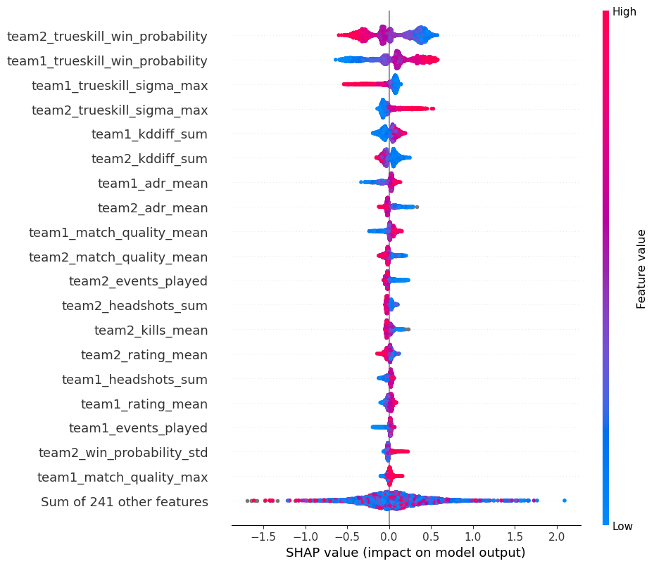
Here is the “beeswarm” view of SHAP values. It shows not just the importance but also how each feature influences the prediction logits9. You can also apply SHAP to individual samples to understand what features caused their prediction logits.
Unsurprisingly, the TrueSkill win probability features are the most important ones. In a sense, this can be seen as a form of stacking, since TrueSkill is another model. Other important features relate to the team’s past performance, like KD ratio and ADR.
Are ~250 features really necessary? Probably not, especially with just 30k samples10. We didn’t do any feature selection, but I’d do permutation importance and adversarial validation on a time split if I had more time on my hands11.
def plot_calibration_curve(y_true, y_pred_proba, set_name, fig, color): mean_predicted_value, fraction_of_positives = calibration_curve(y_true, y_pred_proba, n_bins=10) fig.add_trace(go.Scatter( x=mean_predicted_value, y=fraction_of_positives, mode='lines+markers', name=f'{set_name} set', line=dict(color=color) ))# Create a new figure for the calibration plotcalibration_fig = go.Figure()# Add the perfectly calibrated linecalibration_fig.add_trace(go.Scatter( x=[0, 1], y=[0, 1], mode='lines', name='Perfectly calibrated', line=dict(dash='dot')))# Plot calibration curve for the training setplot_calibration_curve(y_train, model.predict_proba(x_train)[:, 1], 'Training', calibration_fig, 'blue')# Plot calibration curve for the test setplot_calibration_curve(y_test, model.predict_proba(x_test)[:, 1], 'Test', calibration_fig, 'red')# Set layout properties for the calibration plotcalibration_fig.update_layout( title="Calibration plot", xaxis_title="Mean predicted value", yaxis_title="Fraction of positives", xaxis=dict(tickvals=[i/10for i inrange(11)], range=[0, 1]), yaxis=dict(tickvals=[i/10for i inrange(11)], range=[0, 1]), showlegend=True)calibration_fig.show()
The model seems well calibrated (slightly more so on the test set than on the training set, a welcome surprise), which makes it useful for betting: recall from the previous post that our betting decision rule is based on the probability of team 1 or 2 winning. If you use a probability for decision making, it generally needs to be calibrated.
If the model wasn’t well calibrated, we could have used Isotonic regression on a validation set to fix that. There are other options for post-hoc model calibration like Platt scaling, but Isotonic regression works best for tree-based models.
Code
def auc_over_time(df, model, date_col, target_col, features):# Make a copy to avoid modifying the original dataframe and convert match_date to datetime weekly_df = df.copy() weekly_df[date_col] = pd.to_datetime(weekly_df[date_col])# Create a 'week_start_date' column for grouping that represents the start of the week weekly_df['week_start_date'] = weekly_df[date_col].dt.to_period('W').apply(lambda r: r.start_time)# Initialize a dictionary to store AUC for each week weekly_auc = {}for week_start_date, group in weekly_df.groupby('week_start_date'):ifnot group.empty: X = group[features] y = group[target_col] auc = roc_auc_score(y, model.predict_proba(X)[:, 1]) weekly_auc[week_start_date] = aucreturn pd.Series(weekly_auc)def acc_over_time(df, model, date_col, target_col, features):# Make a copy to avoid modifying the original dataframe and convert match_date to datetime weekly_df = df.copy() weekly_df[date_col] = pd.to_datetime(weekly_df[date_col])# Create a 'week_start_date' column for grouping that represents the start of the week weekly_df['week_start_date'] = weekly_df[date_col].dt.to_period('W').apply(lambda r: r.start_time)# Initialize a dictionary to store AUC for each week weekly_auc = {}for week_start_date, group in weekly_df.groupby('week_start_date'):ifnot group.empty: X = group[features] y = group[target_col] auc = accuracy_score(y, model.predict(X)) weekly_auc[week_start_date] = aucreturn pd.Series(weekly_auc)
Code
# Calculate weekly AUC for training and test setsweekly_auc_train = auc_over_time(dataset_train, model, 'match_date', 'target', features)weekly_auc_test = auc_over_time(dataset_test, model, 'match_date', 'target', features)# Plotting the AUC over time using Plotlytrace0 = go.Scatter( x=weekly_auc_train.index, y=weekly_auc_train.values, mode='lines+markers', name='Training Set', line=dict(color='blue'))trace1 = go.Scatter( x=weekly_auc_test.index, y=weekly_auc_test.values, mode='lines+markers', name='Test Set', line=dict(color='red'))layout = go.Layout( title='AUC Over Time', xaxis=dict(title='Week Start Date'), yaxis=dict(title='AUC'), showlegend=True)fig = go.Figure(data=[trace0, trace1], layout=layout)fig.add_hline(y=0.5, line_dash="dash", line_color="black", annotation_text="Random prediction", annotation_position="bottom right")avg_train_auc = weekly_auc_train.mean()avg_test_auc = weekly_auc_test.mean()# Training set average line for the training periodfig.add_shape(type='line', x0=weekly_auc_train.index.min(), y0=avg_train_auc, x1=weekly_auc_train.index.max(), y1=avg_train_auc, line=dict(dash='dash', color='blue', width=2), xref='x', yref='y')# Test set average line for the test periodfig.add_shape(type='line', x0=weekly_auc_test.index.min(), y0=avg_test_auc, x1=weekly_auc_test.index.max(), y1=avg_test_auc, line=dict(dash='dash', color='red', width=2), xref='x', yref='y')# Add annotations for the averagesfig.add_annotation(x=weekly_auc_train.index.max(), y=avg_train_auc, text=f"Train Avg: {avg_train_auc:.2f}", showarrow=False, yshift=10, bgcolor="white")fig.add_annotation(x=weekly_auc_test.index.max(), y=avg_test_auc, text=f"Test Avg: {avg_test_auc:.2f}", showarrow=False, yshift=10, bgcolor="white")fig.show()
There is a train-test performance gap, which implies overfitting, but that’s not a big concern per se. What we really care about is the out-of-time performance, which will also be evaluated with the backtest below. Overfitting is not uncommon in gradient-boosted trees models, but its generalization performance tends to still be better than other models like logistic regression or random forests (I will leave model comparison as an exercise to the reader).
Also, note that there is a big drop in the last 3 weeks of the test dataset. That is exactly when I lost most money! There was some kind of drift or event in that period which made the model perform much worse. That also suggests we should not let the model go fora a long time without re-training. Unfortunately, when we first started to place the bets, those last weeks of the test set were not available to us, being future yet unseen data.
Code
# Calculate weekly AUC for training and test setsweekly_acc_train = acc_over_time(dataset_train, model, 'match_date', 'target', features)weekly_acc_test = acc_over_time(dataset_test, model, 'match_date', 'target', features)# Plotting the AUC over time using Plotlytrace0 = go.Scatter( x=weekly_acc_train.index, y=weekly_acc_train.values, mode='lines+markers', name='Training Set', line=dict(color='blue'))trace1 = go.Scatter( x=weekly_acc_test.index, y=weekly_acc_test.values, mode='lines+markers', name='Test Set', line=dict(color='red'))layout = go.Layout( title='Accuracy Over Time', xaxis=dict(title='Week Start Date'), yaxis=dict(title='Accuracy'), showlegend=True)fig = go.Figure(data=[trace0, trace1], layout=layout)fig.add_hline(y=0.5, line_dash="dash", line_color="black", annotation_text="Random prediction", annotation_position="bottom right")avg_train_acc = weekly_acc_train.mean()avg_test_acc = weekly_acc_test.mean()# Training set average line for the training periodfig.add_shape(type='line', x0=weekly_acc_train.index.min(), y0=avg_train_acc, x1=weekly_acc_train.index.max(), y1=avg_train_acc, line=dict(dash='dash', color='blue', width=2), xref='x', yref='y')# Test set average line for the test periodfig.add_shape(type='line', x0=weekly_acc_test.index.min(), y0=avg_test_acc, x1=weekly_acc_test.index.max(), y1=avg_test_acc, line=dict(dash='dash', color='red', width=2), xref='x', yref='y')# Add annotations for the averagesfig.add_annotation(x=weekly_acc_train.index.max(), y=avg_train_acc, text=f"Train Avg: {avg_train_acc:.2f}", showarrow=False, yshift=10, bgcolor="white")fig.add_annotation(x=weekly_acc_test.index.max(), y=avg_test_acc, text=f"Test Avg: {avg_test_acc:.2f}", showarrow=False, yshift=10, bgcolor="white")fig.show()
The accuracy plot is is similar to AUC in almost all aspects. Note that we’re much better than predicting at random, but that is not a good baseline here. A much better baseline would be the accuracy calculated with the probabilities implied by the betting odds.
Backtesting
Past performance is no guarantee of future results.
Backtesting is replaying the past with your model decisions. One example of backtesting is the following:
Train model with data up to a certain date
Sample betting odds for the next matches
Make bets for those next matches according to your betting strategy
Repeat 1-3 until you cover all the test data
Evaluate ML metrics (e.g. AUC) and business metrics (e.g ROI) on your bets
Backtesting allows us to assess our financial performance, which matters a lot more than ML metrics. For example, is an AUC of 0.77 good or bad? That is hard to tell in general, while a ROI of 1.1 is something we can understand and compare to other strategies (including leaving your money in the bank to earn risk-free interest).
Here, we only assess the ROI of the bets, not other financial metrics like the Sharpe ratio or max drawdown.
For simplicity, we just train the model once and keep it fixed for all future bets, which makes it a more conservative backtest. Also, to make it simple and more conservative, we sample betting odds at random, while in practice we have access to more than one betting odd per match.
First, let’s download the dataset with matches with betting odds:
Only bet if the probability of winning is over 50%
Only bet if the probability of winning is greater than the implied probability by the odds plus a delta of 1%
The bet can either be a fixed amount or determined by the Kelly criterion (here, for simplicity, I only show fixed betting – see previous blog post for a discussion on the Kelly criterion and some variants)
Using the notation from the previous post, here are the betting equations:
There was some trial and error involved in designing our betting strategy and I’m sure there is room for improvement. The delta of 1% is our safety margins due to model error and we found it with a grid search. It’s a parameter you can play with in the simulation below:
The ROI after 2 months is 10%, which annualized would be 63%, not bad at all! For reference, the risk free interest rate in the US today is around 5% per year, while the average S&P500 returns are roughly 10% a year.
We did have an edge after all, or so it seemed. Let’s see the uncertainty across multiple simulations, where the randomness comes from sampling different betting odds for each match:
Code
# Create a Plotly figurefig = go.Figure()# Add traces for each sample's cumulative profitsfor sample_data in all_samples_data:# Make sure to sort the sample_data by 'match_date' sample_data_sorted = sample_data.sort_values(by='match_date') fig.add_trace(go.Scatter( x=sample_data_sorted['match_date'], y=sample_data_sorted['profit'].cumsum(), mode='lines', line=dict(width=1, color='lightgrey'), showlegend=False ))# Add a trace for the average cumulative profits per datefig.add_trace(go.Scatter( x=daily_profit_sum['match_date'], y=daily_profit_sum['cumulative_profit'], mode='lines', name='Avg Cum. Profits', line=dict(width=3, color='blue')))# Adding ROI textfig.add_trace(go.Scatter( x=[daily_profit_sum['match_date'].iloc[-1] + pd.DateOffset(days=4)], y=[daily_profit_sum['cumulative_profit'].iloc[-1]], text=[f"ROI: {roi:.2f}"], # The ROI text mode="text", showlegend=False, textfont=dict( # Adjust the font properties here size=14, color='black', )))# Update layout to add titles and make it more informativefig.update_layout( title="Cumulative Profits over Time with Average", xaxis_title="Match Date", yaxis_title="Cumulative Profit", legend_title="Legend", template="plotly_white", xaxis=dict(type='date'# Ensure that x-axis is treated as date ))# Show the figurefig.show()